Note

This tutorial was generated from a Jupyter notebook that can be downloaded here.

Analyzing Open MDC data

In this tutorial we will use enterprise to analyze open MDC dataset 1.

Get par and tim files

The first step in the process is getting the open MDC1 par and tim files in the tests directory.

parfiles = sorted(glob.glob(datadir + '/*.par'))
timfiles = sorted(glob.glob(datadir + '/*.tim'))

Load pulsars into `Pulsar` objects

enterprise uses a specific Pulsar object to store all of the relevant pulsar information (i.e. TOAs, residuals, error bars, flags, etc) from the timing package. Eventually enterprise will support both PINT and tempo2; however, for the moment it only supports tempo2 through the libstempo package. This object is then used to initalize Signals that define the generative model for the pulsar residuals. This is in keeping with the overall enterprise philosophy that the pulsar data should be as loosley coupled as possible to the pulsar model.

psrs = []
for p, t in zip(parfiles, timfiles):
    psr = Pulsar(p, t)
    psrs.append(psr)

Setup and run a simple noise model on a single pulsar

Here we will demonstrate how to do a simple noise run on a single pulsar. In this analysis we will simply model the noise via a single EFAC parameter and a power-law red noise process.

Set up model

Here we see the basic enterprise model building steps:

Define parameters and priors (This makes use of the Parameter class factory)
Set up the signals making use of the Signal class factories.
Define the model by summing the individual Signal classes.
Define a PTA by initializing the signal model with a Pulsar object.

Notice that powerlaw is uses as a Function here.

##### parameters and priors #####

# Uniform prior on EFAC
efac = parameter.Uniform(0.1, 5.0)

# red noise parameters
# Uniform in log10 Amplitude and in spectral index
log10_A = parameter.Uniform(-18,-12)
gamma = parameter.Uniform(0,7)

##### Set up signals #####

# white noise
ef = white_signals.MeasurementNoise(efac=efac)

# red noise (powerlaw with 30 frequencies)
pl = utils.powerlaw(log10_A=log10_A, gamma=gamma)
rn = gp_signals.FourierBasisGP(spectrum=pl, components=30)

# timing model
tm = gp_signals.TimingModel()

# full model is sum of components
model = ef + rn + tm

# initialize PTA
pta = signal_base.PTA([model(psrs[0])])

We can see which parameters we are going to be searching over with:

print(pta.params)

["J0030+0451_efac":Uniform(0.1,5.0), "J0030+0451_gamma":Uniform(0,7), "J0030+0451_log10_A":Uniform(-18,-12)]

Get initial parameters

We will start our MCMC chain at a random point in parameter space. We accomplish this by setting up a parameter dictionary using the name and sample methods for each Parameter.

xs = {par.name: par.sample() for par in pta.params}
print(xs)

{u'J0030+0451_efac': 4.7352650698633516, u'J0030+0451_gamma': 3.8216965873513029, u'J0030+0451_log10_A': -15.161366939011094}

Note that the rest of the analysis here is dependent on the sampling method and not on enterprise itself.

Set up sampler

Here we are making use of the PTMCMCSampler package for sampling. For this sampler, as in many others, it requires a function to compute the log-likelihood and log-prior given a vector of parameters. Here, these are supplied by PTA as pta.get_lnlikelihood and pta.get_lnprior.

# dimension of parameter space
ndim = len(xs)

# initial jump covariance matrix
cov = np.diag(np.ones(ndim) * 0.01**2)

# set up jump groups by red noise groups
ndim = len(xs)
groups  = [range(0, ndim)]
groups.extend([[1,2]])

# intialize sampler
sampler = ptmcmc(ndim, pta.get_lnlikelihood, pta.get_lnprior, cov, groups=groups,
                 outDir='chains/mdc/open1/')

Sample!

# sampler for N steps
N = 100000
x0 = np.hstack(p.sample() for p in pta.params)
sampler.sample(x0, N, SCAMweight=30, AMweight=15, DEweight=50)

Finished 10.00 percent in 7.578883 s Acceptance rate = 0.27876Adding DE jump with weight 50
Finished 99.00 percent in 77.849424 s Acceptance rate = 0.404505
Run Complete

Examine chain output

We see here that we have indeed recovered the injected values!

chain = np.loadtxt('chains/mdc/open1/chain_1.txt')
pars = sorted(xs.keys())
burn = int(0.25 * chain.shape[0])

truths = [1.0, 4.33, np.log10(5e-14)]
corner.corner(chain[burn:,:-4], 30, truths=truths, labels=pars);

Run full PTA GWB analysis

Here we will use the full 36 pulsar PTA to conduct a search for the GWB. In this analysis we fix the EFAC=1 for simplicity (and since we already know the answer!). This shows an example of how to use Constant parameters in enterprise.

Here you notice some of the simplicity of enterprise. For the most part, setting up the model for the full PTA is identical to that for one pulsar. In this case the only differences are that we are specifying the timespan to use when setting the GW and red noise frequencies and we are including a FourierBasisCommonGP signal, which models the GWB spectrum and spatial correlations.

After this setup, the rest is nearly identical to the single pulsar run above.

# find the maximum time span to set GW frequency sampling
tmin = [p.toas.min() for p in psrs]
tmax = [p.toas.max() for p in psrs]
Tspan = np.max(tmax) - np.min(tmin)

##### parameters and priors #####

# white noise parameters
# in this case we just set the value here since all efacs = 1
# for the MDC data
efac = parameter.Constant(1.0)

# red noise parameters
log10_A = parameter.Uniform(-18,-12)
gamma = parameter.Uniform(0,7)

##### Set up signals #####

# white noise
ef = white_signals.MeasurementNoise(efac=efac)

# red noise (powerlaw with 30 frequencies)
pl = utils.powerlaw(log10_A=log10_A, gamma=gamma)
rn = gp_signals.FourierBasisGP(spectrum=pl, components=30, Tspan=Tspan)

# gwb
# We pass this signal the power-law spectrum as well as the standard
# Hellings and Downs ORF
orf = utils.hd_orf()
crn = gp_signals.FourierBasisCommonGP(pl, orf, components=30, name='gw', Tspan=Tspan)

# timing model
tm = gp_signals.TimingModel()

# full model is sum of components
model = ef + rn + tm  + crn

# initialize PTA
pta = signal_base.PTA([model(psr) for psr in psrs])

Set up sampler

# initial parameters
xs = {par.name: par.sample() for par in pta.params}

# dimension of parameter space
ndim = len(xs)

# initial jump covariance matrix
cov = np.diag(np.ones(ndim) * 0.01**2)

# set up jump groups by red noise groups
ndim = len(xs)
groups  = [range(0, ndim)]
groups.extend(map(list, zip(range(0,ndim,2), range(1,ndim,2))))

sampler = ptmcmc(ndim, pta.get_lnlikelihood, pta.get_lnprior, cov, groups=groups,
                 outDir='chains/mdc/open1_gwb/')

# sampler for N steps
N = 100000
x0 = np.hstack(p.sample() for p in pta.params)
sampler.sample(x0, N, SCAMweight=30, AMweight=15, DEweight=50)

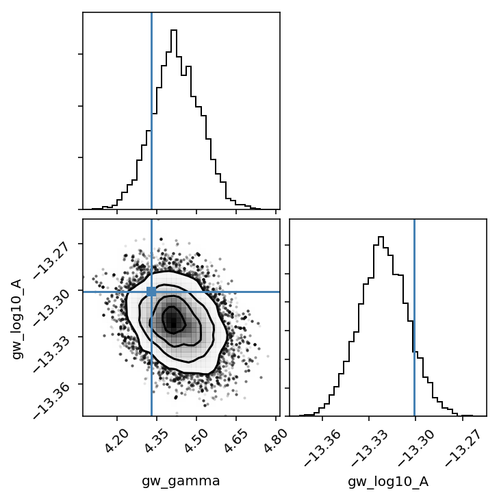
Plot output

chain = np.loadtxt('chains/mdc/open1_gwb/chain_1.txt')
pars = sorted(xs.keys())
burn = int(0.25 * chain.shape[0])

corner.corner(chain[burn:,-6:-4], 40, labels=pars[-2:], smooth=True, truths=[4.33, np.log10(5e-14)]);

Analyzing Open MDC data

Get par and tim files

Load pulsars into Pulsar objects

Setup and run a simple noise model on a single pulsar

Set up model

Get initial parameters

Set up sampler

Sample!

Examine chain output

Run full PTA GWB analysis

Set up sampler

Plot output

Load pulsars into `Pulsar` objects